Imagery for the Santa Ana Wildlife Refuge:
Maps and aerial or satellite imagery are a vital part of any research, conservation or restorative effort. The images below are provided to present the reader with a historic and current view on the Santa Ana Wildlife Refuge area. Additionally, a variety of images were "processed" to illustrate different and distinct features within the park and surrounding environment. Utilizing different methods of image processing provides a way in which to view the evolution of the landscape, vegetation and water ways throughout the area as well as the impact of development for urban or agricultural purposes.
Geotiff sets A-D were compiled in native format TM 4-5 from the USGS Glovis web viewer. Each set was processed in IDRISI for a variety of outcomes focusing on the area in and around Hidalgo County, Texas Santa Ana Wildlife Refuge. The images collected in 1986 show cloud cover directly over the Santa Ana. The overall tile is subject to 10% or less however the area of Santa Ana has been somewhat obscured by the represented 10%. This does provide an opportunity to see the distinction between ground cover and cloud cover in the various processed sets. See each set below for details.
Geotiff sets A-D were compiled in native format TM 4-5 from the USGS Glovis web viewer. Each set was processed in IDRISI for a variety of outcomes focusing on the area in and around Hidalgo County, Texas Santa Ana Wildlife Refuge. The images collected in 1986 show cloud cover directly over the Santa Ana. The overall tile is subject to 10% or less however the area of Santa Ana has been somewhat obscured by the represented 10%. This does provide an opportunity to see the distinction between ground cover and cloud cover in the various processed sets. See each set below for details.
Historic Mapping:
Images spanning almost forty years show the migration of the river from 1939 to 1977 creating new oxbow areas (Resaca) along the refuge boundary.
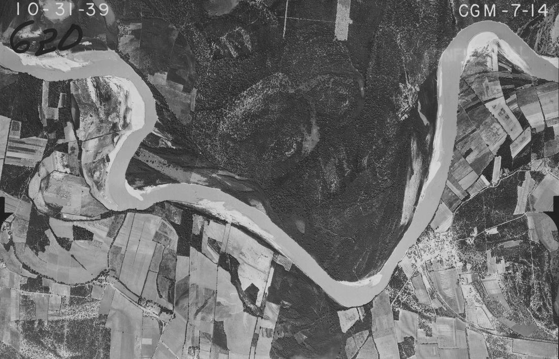
Santa Ana 1939: TNRIS
|
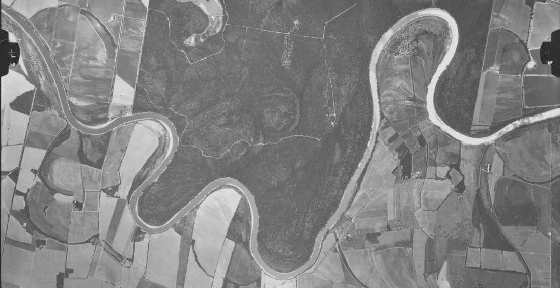
Santa Ana 1977: TNRIS
|
Image Processing: (TM 4-5, dates and 10% or less cloud cover, GLOVIS GeoTIFF- IDRISI processed, North orientation)
2010 Flooding
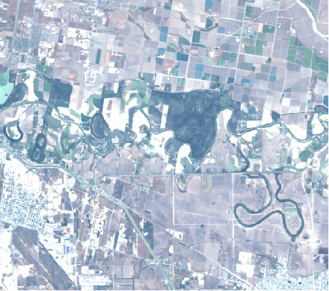
Image A
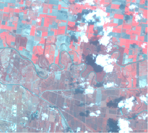
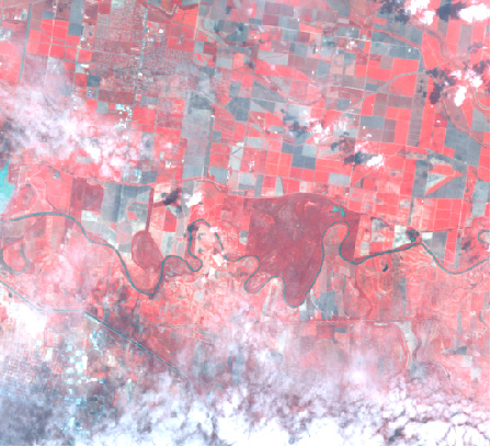
Before and after of the Rio Grande Valley 2010 flooding and after for 2011. Please see Interview with Jennifer Owen-White for additional information on the 2010 flooding as well as information provided on the Santa Ana page of this website.
Image processed as Color Plate 5-2d (Text: Introductory Digital Image Processing: A Remote Sensing Perspective) "B and C" Images (below)- Band 2= Blue, Band 4= Green and Band 7= Red. Vegetation is shown in variations of green throughout the valley and north in agricultural plots. Light purple to dark blue delineates water features while pink to magenta represent urban landscapes. Moisture content is highly visible in the dark blue, darker purple to brown areas in both the 2010 and 2011 images. Large patchy areas of white are indicative of newly eroded areas or sand deposition both a possible result of flooding. The light blue may reflect turbidity of water with suspended sediments. Image A (left) is an alternate view composed in Natural Color for comparison. Natural Color utilizes Band 1= Blue, Band 2= Green and Band 3= Red.
Image processed as Color Plate 5-2d (Text: Introductory Digital Image Processing: A Remote Sensing Perspective) "B and C" Images (below)- Band 2= Blue, Band 4= Green and Band 7= Red. Vegetation is shown in variations of green throughout the valley and north in agricultural plots. Light purple to dark blue delineates water features while pink to magenta represent urban landscapes. Moisture content is highly visible in the dark blue, darker purple to brown areas in both the 2010 and 2011 images. Large patchy areas of white are indicative of newly eroded areas or sand deposition both a possible result of flooding. The light blue may reflect turbidity of water with suspended sediments. Image A (left) is an alternate view composed in Natural Color for comparison. Natural Color utilizes Band 1= Blue, Band 2= Green and Band 3= Red.
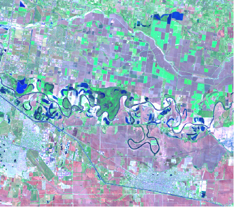
Image B: October 2010 Flood Conditions
Color Plate 5-2d
|
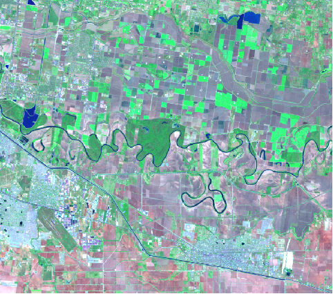
Image C: October 2011 Recovery ProgressColor Plate 5-2d
|
SET A, Traditional False-Color Comp: 1986, 2001 & 2011
A traditional False-Color composition as pictured below shows active vegetation in red, urban and human made structures in white. Inactive vegetation is represented in a variety of grey tones and water features are slightly blue-grey. Cloud cover appears white and shadows corresponding on the ground are dark grey-black. October 2011 shows significantly less vegetative cover in the vicinity of the refuge as well as in the outlying agricultural fields. Color band sequence is Band 1= Blue, Band 4= Red and Band 2= Green all processed in COMPOSITION frame of IDRISI.
Santa Ana: July 1986 False Color Comp
|
Santa Ana: October 2001 False Color Comp
|
Santa Ana: October 2011 False Color Comp
|
SET B, Near-Infrared (False Color) Comp: 1986, 2001 & 2011
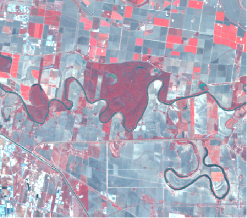
Active vegetation, as is with the Traditional False-Color palette, is shown in green when utilizing a Near-Infrared band sequence. Inactive vegetation (but perhaps more saturated soil conditions) is shown in a gradient of purple to pink while human made structures as well as cloud cover appears white. October 2001 shows a particularly active growth cycle and moderate to heavy cloud cover to the south of the image frame. Also evident is the growth in urban areas located to the southwest between 1986 and 2011. Color band sequence is Band 1= Blue, Band 4= Green and Band 2= Red all processed in COMPOSITION frame of IDRISI.
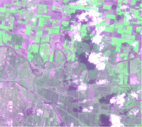
Santa Ana: July 1986 Near Infrared
|
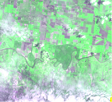
Santa Ana: October 2001 Near Infrared
|
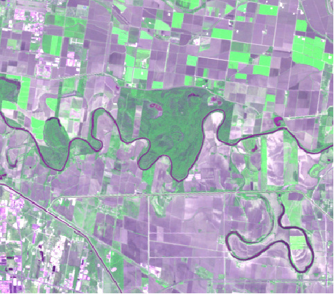
Santa Ana: October 2011 Near Infrared
|
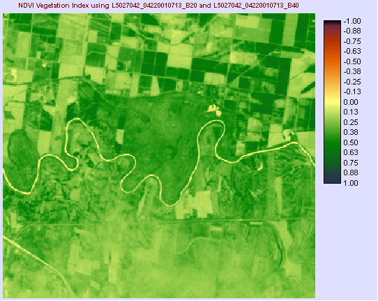
SET C, NDVI: Vegetation Index: 1986, 2001 & 2011
NDVI (Normalized Difference Vegetation Index) values range from 1 to -1 as demonstrated on the scale to the right of the images below and are utilized to exhibit vegetation growth. Vegetation in the area ranges from .63 to just above 0.0 on the NDVI index scale. Negative numbers indicate little to zero vegetation. The Rio Grande flowing through the refuge displays negative values in the -.38 to -.75 range. Cloud cover in the 1986 and 2001 images are a zero value as well.
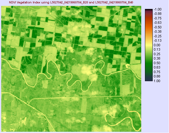
Santa Ana: July 1986 NDVI
|
Santa Ana: October 2001 NDVI
|
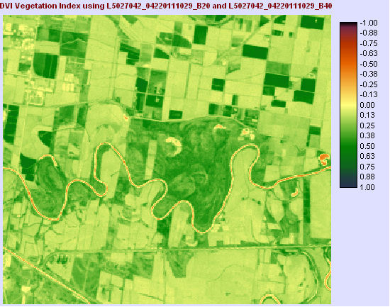
Santa Ana: October 2011 NDVI
|
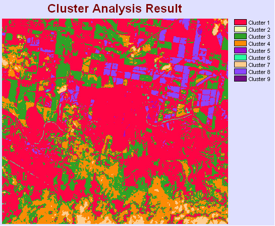
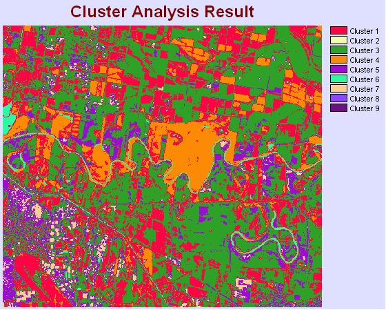
SET D, Cluster Analysis: 1986, 2001 & 2011
Cluster analysis provides a way to group image cells in order to highlight distributive patterns based on their similar numerical value. Different elements will provide a different signature color to be interpreted. Nine CLUSTERS are identified in each image. The predominant CLUSTER values are described below by year. Between 1986 and 2011 a dramatic increase in the variation of CLUSTERS is apparent.
1986: Red values (Cluster 1) appear to be active vegetation. Purple (Cluster 8) and green (Clusters 3 & 6) indicate cloud cover while orange (Cluster 4) represents humane made features and possibly areas of inactive vegetation.
2001: Cloud cover to the south and south central of the image is represented in green (Cluster 3) and orange (Cluster 4). Red (Cluster 1) is active vegetation or saturated conditions. Purple (Cluster 8) is agricultural land as seen in the distinctive parcel shapes.
2011: Many more distinct cell CLUSTERS are visible in 2011. Orange (Cluster 4), Red (Cluster 1) represent active vegetation or moist soil conditions. Clusters 3 and 8 show less active vegetation areas while Clusters 9 and 2 demonstrate human structures and/ or paved areas as is apparent in the mid-bottom left of the image.
Through IDRISI a CLUSTER analysis was preformed utilizing bands 1-4 for each year if imagery (1986-2011).
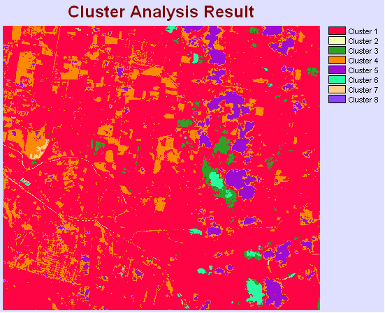
Santa Ana: July 1986 CLUSTER
|
Santa Ana: October 2001 CLUSTER
|
Santa Ana: October 2011 CLUSTER
|
